This workbook is an introduction to the basic concepts and designs relating to the paper
Fast estimation of sparse quantum noise by Harper, Yu and Flammia (in production)
This workbook is going to go through the basic ideas behind the Walsh Hadamard Transform for a 2 qubit system. I will focus on the type of transforms, and how it relates eigenvalues (fidelities) and probabilities and measurement outcomes.
Copyright 2020: Robin Harper
Software needed
For this introductory notebook, we need minimal software. All these packages should be available through the Julia package manager.
If you get an error trying to "use" them the error message tells you how to load them.
using Hadamard

# convenience (type /otimes<tab>) - <tab> is the "tab" key.
⊗ = kron
# type /oplus<tab>
⊕ = (x,y)->mod.(x+y,2)
Some preliminary information
Conventions
What's in a name?
There are a number of conventions as to where which qubit should be. Here we are going to adopt a least significant digit approach - which is different from the normal 'ket' approach.
So for example: $IZ$ means an $I$ 'Pauli' on qubit = 2 and a $Z$ 'Pauli' on qubit = 1 (indexing off 1).
Arrays indexed starting with 1.
For those less familiar with Julia, unlike - say - python all arrays and vectors are indexed off 1. Without going into the merits or otherwise of this, we just need to keep it in mind. With our bitstring the bitstring 0000 represents the two qubits $II$, it has value 0, but it will index the first value in our vector i.e. 1.
Representing Paulis with bitstrings.
There are many ways to represent Paulis with bit strings, including for instance the convention used in Improved Simulation of Stabilizer Circuits, Scott Aaronson and Daniel Gottesman, arXiv:quant-ph/0406196v5.
Here we are going to use one that allows us to naturally translate the Pauli to its position in our vector of Pauli eigenvalues (of course this is arbitrary, we could map them however we like).
The mapping I am going to use is this (together with the least significant convention):
- I $\rightarrow$ 00
- X $\rightarrow$ 01
- Y $\rightarrow$ 10
- Z $\rightarrow$ 11
This then naturally translates as below:
SuperOperator - Pauli basis
We have defined our SuperOperator basis to be as below, which means with the julia vector starting at 1 we have :
| Pauli | Vector Index | --- | Binary | Integer |
|---|---|---|---|---|
| II | 1 | → | 0000 | 0 |
| IX | 2 | → | 0001 | 1 |
| IY | 3 | → | 0010 | 2 |
| IZ | 4 | → | 0011 | 3 |
| XI | 5 | → | 0100 | 4 |
| XX | 6 | → | 0101 | 5 |
| XY | 7 | → | 0110 | 6 |
| XZ | 8 | → | 0111 | 7 |
| YI | 9 | → | 1000 | 8 |
| YX | 10 | → | 1001 | 9 |
| YY | 11 | → | 1010 | 10 |
| YZ | 12 | → | 1011 | 11 |
| ZI | 13 | → | 1100 | 12 |
| ZX | 14 | → | 1101 | 13 |
| ZY | 15 | → | 1110 | 14 |
| ZZ | 16 | → | 1111 | 15 |
I have set this out in painful detail, because its important to understand the mapping for the rest to make sense.
So for instance in our EIGENVALUE vector (think superoperator diagonal, or what we used to call the Pauli fidelities), the PAULI $YX$ has binary representation $Y$=10 $X$=01, therefore 1001, has "binary-value" 9 and is the 10th (9+1) entry in our eigenvalue vector.
What's in a Walsh Hadamard Transform?
The standard Walsh-Hadmard transform is based off tensor (Kronecker) products of the following matrix:
$$\left(\begin{array}{cc}1 & 1\\1 & -1\end{array}\right)^{\otimes n}$$WHT_natural
So for one qubit it would be:
$\begin{array}{cc} & \begin{array}{cccc} \quad 00 & \quad 01 & \quad 10 &\quad 11 \end{array}\\ \begin{array}{c} 00\\ 01\\ 10\\11\end{array} & \left(\begin{array}{cccc} \quad 1&\quad 1& \quad 1 &\quad 1\\ \quad 1 &\quad -1 & \quad 1 &\quad -1\\ \quad 1&\quad 1 & \quad -1 &\quad -1\\ \quad 1 &\quad -1 & \quad -1 &\quad 1\\\end{array}\right) \end{array}$
where I have included above (and to the left) of the transform matrix the binary representations of the position and the matrix can also be calculated as $(-1)^{\langle i,j\rangle}$ where the inner product here is the binary inner product $i,j\in\mathbb{F}_2^n$ as $\langle i,j\rangle=\sum^{n-1}_{t=0}i[t]j[t]$ with arithmetic over $\mathbb{F}_2$
WHT_Pauli
In the paper we use a different form of the Walsh-Hadamard transform. In this case we use the inner product of the Paulis, not the 'binary bitstring' inner product. The matrix is subtly different some rows or, if you prefer, columns are swapped:
$\begin{array}{cc} & \begin{array}{cccc} I(00) & X(01) & Y(10) & Z(11) \end{array}\\ \begin{array}{c} I(00)\\ X(01)\\ Y(10)\\Z(11)\end{array} & \left(\begin{array}{cccc} \quad 1&\quad 1& \quad 1 &\quad 1\\ \quad 1 &\quad 1 & \quad -1 &\quad -1\\ \quad 1&\quad -1 & \quad 1 &\quad -1\\ \quad 1 &\quad -1 & \quad -1 &\quad 1\\\end{array}\right) \end{array}$
To calculate this one, we can use the 'symplectic inner product' to work it out. In particular for one of the indices you just need to swap the X and Y components. A matrix of the form
$$\begin{align} J_n = \mathbf{I}_n\otimes X = \left(\begin{smallmatrix} 0 & 1 & & & \\ 1 & 0 & & & \\ & & \ddots & & \\ & & & 0 & 1 \\ & & & 1 & 0 \end{smallmatrix}\right), \end{align}$$will do this and then use the binary inner product between the index and the transformed index. (The binary inner is detailed above).
Which one to use
When transforming Pauli eigenvalue to the probability of a particular error occuring, there are distinct advantages in using the WHT_Pauli transform. The order of the Pauli errors and the order of the Pauli eigenvalues remains the same. However, most common packages (including the one we are going to use here in Julia) don't support this type of transform, rather they implement the WHT_natural transform. The WHT_natural transform also makes the peeling algorithm slightly less fiddly. However it does mean we need to be very careful about the order of things. If we use the WHT_natural transform then the following relationship holds - note the indices (labels) of the Paulis in the probability vector:
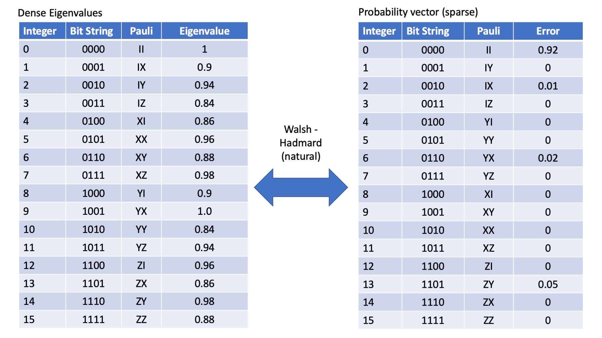
So the natural translation (labelling of Paulis) then becomes as follows:
Eigenvalue vector space
- I $\rightarrow$ 00
- X $\rightarrow$ 01
- Y $\rightarrow$ 10
- Z $\rightarrow$ 11
Probability vector space
- I $\rightarrow$ 00
- X $\rightarrow$ 10
- Y $\rightarrow$ 01
- Z $\rightarrow$ 11
The numbers here are the numbers from a previous example (with sparse errors) - for the purposes of demonstrating the next step, I'll use a denser probability distribution.
Set up some Pauli Errors to demonstrate
# TO demonstrate the peeling decoder we are going to set up a sparse (fake) distribution.
# This is going to mirror the example shown above -
# NOTE Julia indexing starts at 1, so we add 1 to the integers in the above table
# TO demonstrate the peeling decoder we are going to set up a sparse (fake) distribution.
# This is going to be a 4 qubit (so 4^4 = 256 possible probabilities)

dist = zeros(16)
cl = zeros(2,4)

# Qubit 1
cl[1,2] = 0.01 #y1
cl[1,3] = 0.004 #x1
cl[1,4] = 0.001 #z1
cl[1,1] = 1-sum(cl[1,:])

# Qubit 2
cl[2,2] = 0.03
cl[2,3] = 0.02
cl[2,4]=  0.005
cl[2,1] = 1-sum(cl[2,:])

for q1 in 1:4
    for q2 in 1:4
      dist[(q2-1)*4+q1] = cl[1,q1]*cl[2,q2]
    end
end

# rounding to 10 digits just to get rid of some annoying numerical instability
dist = round.(dist,digits=10)
basicSuperOpDiagonal = round.(ifwht_natural(dist),digits=10)
print("Basic SuperOperator (diagonal): $basicSuperOpDiagonal\n")
print("Distribution: $(dist)\n")
So why do we need the transform.
There are two main reasons:
- We can determine the eigenvalues in a SPAM (state preperation and measurement) error free way. This uses the technicques of randomised benchmarking and is listed later.
- We can't actually deteremine the probabilities directly - but we can determine the eigenvalues.
Why do I say we can't determine the probabilities directly?
How to work out what we "measure"
Well we can only measure a commuting set of probabilities simultaneously (as otherwise the measurement alters the state). So for instance if we prepare in the computational basis $|00\rangle\langle00|$, and measure the overlap between the noise altered state and the different computational basis states we get a probability distribution of the chance of observing an error.
So our measurements here are a projective basis.
$M_{00}=|00\rangle\langle00|,M_{01}=|01\rangle\langle01|,M_{10}=|10\rangle\langle10|,M_{11}=|11\rangle\langle11|$
Which you should be able to convince yourself form the following density matrices:
$M_{00}=\left(\begin{array}{cc}1&0&0&0\\0&0&0&0\\0&0&0&0\\0&0&0&0\end{array}\right), M_{01}=\left(\begin{array}{cc}0&0&0&0\\0&1&0&0\\0&0&0&0\\0&0&0&0\end{array}\right),M_{10}=\left(\begin{array}{cc}0&0&0&0\\0&0&0&0\\0&0&1&0\\0&0&0&0\end{array}\right),M_{11}=\left(\begin{array}{cc}0&0&0&0\\0&0&0&0\\0&0&0&0\\0&0&0&1\end{array}\right)$
(note they sum to the identity matrix - see Neilson & Chuang as to why this is a POVM).
And if we vectorise these in the Pauli basis we get the following:
$(M_{00}|=\left(\begin{array}{*{11}c} 1 & 0 & 0 & 1 & 0 & 0 & 0 & 0 & 0 & 0 & 0 & 0 & 1 & 0 & 0 & 1 &\end{array}\right)$
$(M_{01}|=\left(\begin{array}{*{11}c} 1 & 0 & 0 & -1 & 0 & 0 & 0 & 0 & 0 & 0 & 0 & 0 & 1 & 0 & 0 & -1 \end{array}\right)$
$(M_{10}|=\left(\begin{array}{*{11}c} 1 & 0 & 0 & 1 & 0 & 0 & 0 & 0 & 0 & 0 & 0 & 0 & -1 & 0 & 0 & -1 \end{array}\right)$
$(M_{11}|=\left(\begin{array}{*{11}c} 1 & 0 & 0 & -1 & 0 & 0 & 0 & 0 & 0 & 0 & 0 & 0 & -1 & 0 & 0 & 1 \end{array}\right)$
Where I have ignored the normalisation factor of 0.25 in front of each of these (Sometimes you will see the normalisation split evenly betweeen the state prep and measurment - i.e 0.5 on both). Basically I'll just divide everything by 4!
The state preperation vector is just
$|\rho_{00})=||00\rangle\langle00|)=\left(\begin{array}{*{11}c} 1 \\ 0 \\ 0 \\ 1 \\ 0 \\ 0 \\ 0 \\ 0 \\ 0 \\ 0 \\ 0 \\ 0 \\ 1 \\ 0 \\ 0 \\ 1 \\ \end{array}\right)$
, so we can see in the absence of noise
$(M_{00}|\rho_{00}) = 1$,$(M_{01}|\rho_{00}) = 0$,$(M_{10}|\rho_{00}) = 0$,$(M_{11}|\rho_{00}) = 0$
which (since they form a basis) is what we would expect.
So how does noise affect this?
zs =
 [[1, 0, 0, 1, 0, 0, 0, 0, 0, 0, 0, 0, 1, 0, 0, 1],
 [1, 0, 0, -1, 0, 0, 0, 0, 0, 0, 0, 0, 1, 0, 0, -1],
 [1, 0, 0, 1, 0, 0, 0, 0, 0, 0, 0, 0, -1, 0, 0, -1],
 [1, 0, 0, -1, 0, 0, 0, 0, 0, 0, 0, 0, -1, 0, 0, 1]]
# Side note if you have installed my Juqst package (see https://github.com/rharper2/Juqst.jl), then
# You can generate these for any size using Juqst.genZs(2) (for 2 qubits).
using LinearAlgebra

superOperatorNoise = diagm(0=>basicSuperOpDiagonal)
If we measure this noise using these measurement operators then we get the following:
# The measurement outcomes are then:
print("M_00 = ↑↑ = $(round(0.25*zs[1]'*superOperatorNoise*zs[1],digits=10))\n")
print("M_01 = ↑↓ = $(round(0.25*zs[2]'*superOperatorNoise*zs[1],digits=10))\n")
print("M_10 = ↓↑ = $(round(0.25*zs[3]'*superOperatorNoise*zs[1],digits=10))\n")
print("M_11 = ↓↓ = $(round(0.25*zs[4]'*superOperatorNoise*zs[1],digits=10))\n")
outcomes = 0.25.*[x'*superOperatorNoise*zs[1] for x in zs]
print("total probability = $(sum(outcomes))\n")
What do these probabilities represent?
Basically if we took a quantum device, prepared the |00$\rangle$ state, subjected it to that noisy channel and then measured the resulting state, we would expect to see the above probability distribution on the measurement results.
One question we might ask then is what would we see if we ran it through the noisy channel twice. Well because we know the noisy channel we can simply apply it twice in simulation and see the new probability distribution.
On an actual device we can only see the probability distribution for $2^n$ commuting measurements at a time - and that makes it a lot more difficult to work the global probability distribution - as we explore now:
So how does this relate to the acutal global distribution we had?
Well at first blush it doesn't if we remember the actual probability distribution looks like this:
# Some function to give us labels:
function probabilityLabels(x;qubits=2)
    str = string(x,base=4,pad=qubits)
    paulis = ['I','Y','X','Z']
    return map(x->paulis[parse(Int,x)+1],str)
end

function fidelityLabels(x;qubits=2)
    str = string(x,base=4,pad=qubits)
    paulis = ['I','X','Y','Z']
    return map(x->paulis[parse(Int,x)+1],str)
end
# Print label and probability
for i in 1:16
    print("$i: $(probabilityLabels(i-1)): $(dist[i])\n")
end
So we can see the IZ pauli error rate is 0.00945, yet we measured updown as 0.0133, what gives?
Well the probability of "seeing" an error in the computational basis is NOT the IZ error rate. In fact we can't see a Z error at all. We can only see an X or a Y error.
Therefore we will see an error on qubit 1 (only) if there is no error seen on qubit 2, and an error seen on qubit 1. The pauli errors that will give us only an error on qubit 1 are:
IX, IY, ZY and ZX (recall qubit 1 is the right most digit).
Those correspond to indices 2,3, 14 and 15 above:
print("Sum of relevant probabilities: $(dist[2]+dist[3]+dist[14]+dist[15])\n")
print("Expected measurement outcome: M_01 = ↑↓ = $(round(0.25*zs[2]'*superOperatorNoise*zs[1],digits=10))\n")
Similarly if we wanted the probability of seeing an error on qubit 2,
XI, YI, YZ, XZ (9,5,8 and 12)
print("Sum of relevant probabilities: $(round(dist[9]+dist[5]+dist[8]+dist[12],digits=10))\n")
print("Expected measurement outcome: M_10 = ↓↑ = $(round(0.25*zs[3]'*superOperatorNoise*zs[1],digits=10))\n")
And finally the chance of seeing an error on BOTH qubits is YX, YY, XX, XY (7,6,11,10)
print("Sum of relevant probabilities: $(round(dist[7]+dist[6]+dist[11]+dist[10],digits=10))\n")
print("Expected measurement outcome: M_11 = ↓↓ = $(round(0.25*zs[4]'*superOperatorNoise*zs[1],digits=10))\n")
But what is the important thing to keep in mind?
Well its that these probabilities (which are made up combinations of the Pauli error rates - transform directly to the appropriate eigenvalue entry). So if we set out the probabilities in a vector and then transform them: We get the entries in the eigenvalue vector.
So the 'measured' proabilities in the computational basis are:
$\left(\begin{array}{c}0.9367\\0.0133\\0.0493\\0.0007\end{array}\right)$
We can use the WHT (natural) transform on this:$\qquad \left(\begin{array}{*{11}c} 1 & 1 & 1 & 1 \\ 1 & -1 & 1 & -1 \\ 1 & 1 & -1 & -1 \\ 1 & -1 & -1 & 1 \\ \end{array}\right)$
To get $\qquad\left(\begin{array}{c}1.0\\0.972\\0.9\\ 0.8748\end{array}\right)$
round.(Hadamard.hadamard(4)*[0.9367, 0.0133, 0.0493, 0.0007],digits=10)
And those are exactly the entries (for II, IZ, ZI and ZZ) in the diagonal of the super operator
# Print label and probability
for i in 1:16
    print("$i: $(fidelityLabels(i-1)): $(basicSuperOpDiagonal[i])\n")
end
So this gives us the way we can reconstruct the Global probability distribution
(which in turn tells us the chance of an X error or Y error or Z error on each qubit, which in turn lets us e.g. fine-tune our error correction decoders)
We can measure each different set of stabiliser measurements until we have reconstructed the entire superoperator (in fact we don't need to do this much work, but that is for another time!)
One final example:
We should be able to see that II, ZX, YZ and XY are all mutually commuting - that means we can in fact measure them all at the same time.
How would that work? Well we just have to find the correct basis. (As always), there are several ways of thinking of this. We can imagine that if we could prepare the following state:
req = [1,0,0,0,0,0,1,0,0,0,0,1,0,1,0,0]
for i in 1:16
    print("$(string(i,pad=2)) $(fidelityLabels(i-1)): $(req[i])\n")
end
Then that is going to pick up the relevant entries from the SuperOperator representation. If we then measure in the same basis we are going to get the correct probabilities, which we can transform back to get the eigenvalues.
Of course because we are just manipulating matrices it all feels a bit 'circular'. In a device where we don't know the eigenvalues, what we have to do is actually run the circuits.
So the circuit that transforms into various stabiliser groups look like this

Here we are interested in (a).
Note
Here I am going to use some code that is available at: github - rharper2/Juqst.jl
using Juqst
# Set up the relevant gates
cnot21 = [1 0;0 1]⊗[1 0;0 0]+ [0 1;1 0]⊗[0 0;0 1]
superCnot21 = makeSuper(cnot21)
superPI = makeSuper([1 0;0 im]⊗[1 0;0 1])
superIP = makeSuper([1 0;0 1]⊗[1 0;0 im])
superHH = makeSuper((1/sqrt(2)*[1 1;1 -1])⊗(1/sqrt(2)*[1 1;1 -1]));
# Circuit (a) is then just these gates applied (here circuit is from left to right, but matrices the other way!)

circuit = superCnot21*superPI*superCnot21*superIP*superHH
And we can apply this to the $|00\rangle$ state, to generate the correct state:
newB = circuit*zs[1]
for i in 1:16
    print("$(string(i,pad=2)) $(fidelityLabels(i-1)): $(newB[i])\n")
end
And the reverse circuit takes it back into the computational basis.
Here I was just going to be lazy and use the transpose of the superoperator gate that represents the circuit, but lets show they are the same. Reverse circuit - just apply inverse gates in reverse order one at a time (recall CNOT is self inverting, and three phases = phase$^\dagger$
Rcircuit = superHH*superIP*superIP*superIP * superCnot21*superPI*superPI*superPI*superCnot21
Rcircuit *circuit
# And just a little sanity check, that the transpose of superoperator is indeed its inverse
Rcircuit == transpose(circuit)
We can work out what stats we would get if we ran this experiment
(this is what we would see in an actual device -- assuming the only noise is our superOperatorNoise)
# The measurement outcomes are then:
print("M_00 = ↑↑ = $(round(0.25*zs[1]'*Rcircuit*superOperatorNoise*circuit*zs[1],digits=10))\n")
print("M_01 = ↑↓ = $(round(0.25*zs[2]'*Rcircuit*superOperatorNoise*circuit*zs[1],digits=10))\n")
print("M_10 = ↓↑ = $(round(0.25*zs[3]'*Rcircuit*superOperatorNoise*circuit*zs[1],digits=10))\n")
print("M_11 = ↓↓ = $(round(0.25*zs[4]'*Rcircuit*superOperatorNoise*circuit*zs[1],digits=10))\n")
outcomes = 0.25.*[x'*Rcircuit*superOperatorNoise*circuit*zs[1] for x in zs]
print("total probability = $(sum(outcomes))\n")
Then we transform back to the eigenvalues:
round.(Hadamard.hadamard(4)*outcomes,digits=10)
# Recall the eigenvalues:
# Print label and probability
for i in 1:16
    print("$i: $(fidelityLabels(i-1)): $(basicSuperOpDiagonal[i])\n")
end
And we can see we have correctly 'reconstructed'
- ZX
- YZ
- XY
As predicted.
We can change the circuits and reconstruct all of the eigenvalues, then we can generate the 'global' probability distribution. There are however otherways of doing this if we can assume e..g the distribution is sparse.